Bare Bones Linear Regression

Code

All code here can be found in this repository.

Introduction

At surface level, machine learning is dauntingly complex. It's not something you can just "slide" into and grasp effortlessly, even with good prerequisites (which I certainly don't have). Here, we're going to implement linear regression from scratch to learn the relationship between two variables which are linearly coorelated using Python and Numpy. That's right, no fancy libraries allowed. Those are for taking shortcuts. Here, I'm solifying my understanding of theory, not implementation.

Dataset

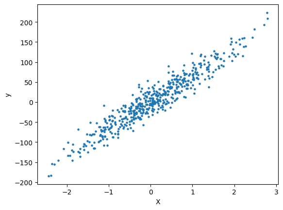
For simplicity, we'll use a two-dimensional linear dataset. Our model will learn the relationship between two variables, \(X\) and \(y\). The datapoints are meaningless and will be generated using scikit-learn's "datasets" library.

We use 500 training samples \(\text{(\(X\),\(y\))}\). Often, \(X\) may have more than one feature (this is especially true for more complex models). However, we only have on input feature \(X_1\). Hence, the dimensions of \(X\) are \(\text{# samples}\ \times \text{# features}\ = 500 \times 1\).

Similarly, \(y\) has only one output variable \(y\). Hence, the dimensions of \(y\) are \(\text{# samples}\ \times \text{# outputs}\ = 500 \times 1\). Here are our two arrays so far:

\[X=\begin{bmatrix}\ a_{1} \\ a_{2} \\ a_{3} \\ \vdots \\ a_{500}\end{bmatrix} y=\begin{bmatrix}\ b_{1} \\ b_{2} \\ b_{3} \\ \vdots \\ b_{500}\end{bmatrix}\]

where \(a\) are input training samples and \(b\) are output training samples.

Here are the training samples \(\text{(\(X\),\(y\))}\) plotted in Matplotlib:

Conventions

We label the inputs or features as \(X\) and the outputs or target variables as \(y\); \(\text{(\(X^{i}\),\(y^{i}\))}\) represents the \(i^{th}\) training sample.

The model's parameters or "weights" are denoted as \(\theta\).

The number of training examples is \(m\). Here, \(m=500\).

The number of features or input variables is \(n\). Here, \(n=1\).

Hypothesis

Recall that we want to creating a mapping from \(X\) to \(y\). Since our data is linear, our mapping is a linear function (or hypothesis) \(h(X)=\theta_{0}X_{0} + \theta_{1}X_{1}\) where \(X_{0}\) is a dummy feature whose value is \(1\). Although unnecessary for our simple case, \(h(X)\) can be written as \(h(X)=\sum_{i=0}^{n} \theta_{i}X_{i}\) for conciseness.

Optimizing \(\theta\)

Now our task is to make \(h\) a good function for finding \(y\) given \(X\). To do this, we can tweak the parameters \(\theta\). We determine how "bad" \(h\) is with our cost function

\[J(\theta)=\frac{1}{2m}\sum_{i=1}^{m}(h_{\theta}(X^{i})-y^{i})^{2}\]

where \(m\) is the number of training examples. The cost function's job is to tell us how far the actual values \(y\) are from \(h\)'s predicted values. \(J(\theta)\) is based on the formula for mean squared error, or MSE:

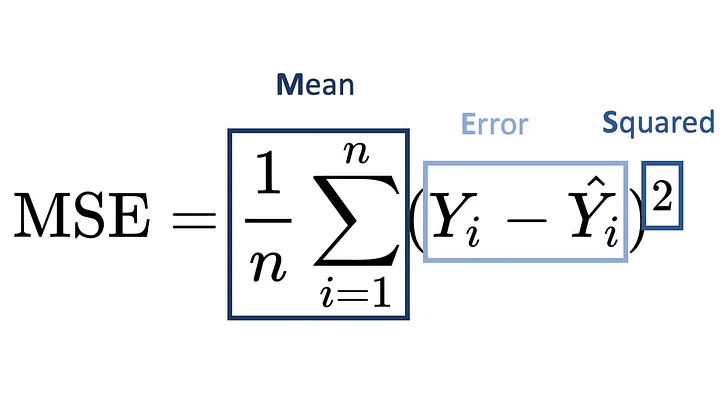
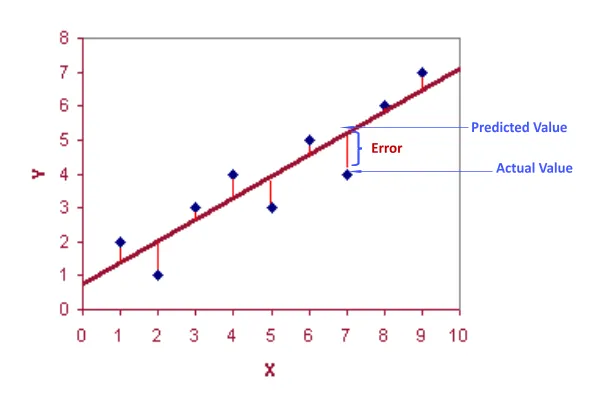
Here's \(J(\theta)\) again in plain language:

\[J(\theta)=\frac{1}{2(\text{# training examples})} \sum_{i=1}^{\text{# training examples}} (\text{predicted output for training sample \(X^{i}\)}- \text{actual output of training sample})^{2}\]

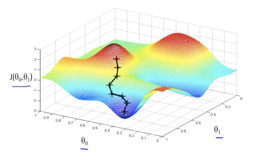
Now our job is to minimize \(J(\theta)\). We'll use an algorithm called gradient descent to minimize \(J(\theta)\). Since we know that \(\theta_{0}\) and \(\theta_{1}\) affect the accuracy of \(h\), we can plot them against our cost function:

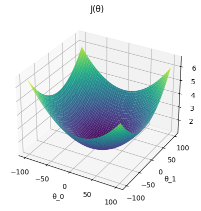
We see that there is an optimal set of parameters \((\theta_{0},\theta_{1})\) that yields a minimal cost \(J(\theta)\). In order to find the optimal location \((\theta_{0},\theta_{1})\), we'll initialize random parameters \(\theta\) and iteratively adjust them towards the global minima.

To determine which direction to move the parameters \(\theta\) in, we'll calculate the direction of steepest ascent, or the gradient \(\nabla J(\theta)\) (the vector containing partial derivatives with respect to each parameter \(\theta\) of \(J(\theta)\)), and move the parameters opposite the gradient.

\[\nabla J(\theta)=[\frac{\partial J}{\theta_{0}}, \frac{\partial J}{\theta_{1}}]\]

Now, we use the update rule \(\theta:=\theta-\alpha\nabla J(\theta)\) where \(\text{:=}\) represents assignment from right to left and \(\alpha\) is the model's learning rate (how significantly the parameters are updated at each step of the gradient descent algorithm).

It turns out, as we run through these iterations, tweaking the parameters of \(h\), the cost function \(J(\theta)\) is minimized (left) and \(h\) becomes a more accurate mapping from \(X\) to \(y\) (right).

if someone actually read this, tysm :p